
My first Monte Carlo
Redo what the film showed in Python, right here.
The code runs in your browser: Python 3.13, NumPy and matplotlib load the first time (about twenty megabytes, cached afterwards). Cells marked with a white bar are yours to complete; the solutions unfold cell by cell.
Shift + Enter runs the cell and moves to the next one.
The class follows the French practical (four missions: Méré, π, the option, the ruin). This English notebook is complementary practice. Open the French practical
Graded assignment
The graded assignment of session 1, « Combien mettre en Bourse ? », is set in French: its brief, kit and experiment are on the French page.
Dynamic Optimization and Monte Carlo Methods in Python — Master 2 MBFA – Financial Engineering and Modelling and Master 2 MBFA – Insurance Engineering, Université Sorbonne Paris Nord. Session 1, “Computing with chance”. Time: about an hour and a half, then challenges for those who are quick.
Goal. Redo the experiments of the film of session 1 yourself, line by line: the coin, π with darts, the bell curve of the estimates that narrows, the confidence interval that “catches” the true value 95 times out of a hundred, and the price of a call option compared with its judge, the Black–Scholes formula.
Rules of the game.
- NumPy only for the computations (and matplotlib for the figures); a single generator,
np.random.default_rng(seed). - Predict, simulate, verify: before each experiment, write down what you expect; then simulate; then compare.
- Colour code of the course: blue = simulated, orange = exact (the judge), red = failure, grey = everything else.
- The cells marked
# TO COMPLETEare for you to fill in. The notebook runs even when incomplete: the checks print “to complete” as long as the answer is missing.
import math
import numpy as np
import matplotlib.pyplot as plt

# Colour code of the course (the same as in the videos, the course notes and the slides)
BLUE, ORANGE, RED, GREY = "#5B9CFF", "#FFA14A", "#FF6B66", "#5F6C84"
plt.rcParams.update({
    "figure.figsize": (7.5, 3.6), "figure.dpi": 100, "axes.grid": True, "grid.color": "#E4E9F1",
    "axes.spines.top": False, "axes.spines.right": False, "axes.edgecolor": "#9AA8BF",
    "axes.titlelocation": "left", "axes.titleweight": "bold", "font.size": 10,
    "axes.prop_cycle": plt.cycler(color=[BLUE, ORANGE, RED, GREY]),
})


def ready(*objects):
    """True if every object has been computed (neither None nor NaN): the notebook runs even when incomplete."""
    for o in objects:
        if o is None or o is Ellipsis:
            return False
        try:
            if np.any(np.isnan(np.asarray(o, dtype=float))):
                return False
        except (TypeError, ValueError):
            pass
    return True


def check(name, value, expected, tol):
    """Compare a value with what is expected (to within tol), without ever interrupting the notebook."""
    if not ready(value):
        print(f"… {name}: to complete")
    elif abs(float(value) - expected) <= tol:
        print(f"✓ {name} = {float(value):.6g} (expected ≈ {expected:.6g})")
    else:
        print(f"✗ {name} = {float(value):.6g}, expected ≈ {expected:.6g} (to within ± {tol:g}): review your code")
import math
import numpy as np
import matplotlib.pyplot as plt
# Colour code of the course (the same as in the videos, the course notes and the slides)
BLUE, ORANGE, RED, GREY = "#5B9CFF", "#FFA14A", "#FF6B66", "#5F6C84"
plt.rcParams.update({
"figure.figsize": (7.5, 3.6), "figure.dpi": 100, "axes.grid": True, "grid.color": "#E4E9F1",
"axes.spines.top": False, "axes.spines.right": False, "axes.edgecolor": "#9AA8BF",
"axes.titlelocation": "left", "axes.titleweight": "bold", "font.size": 10,
"axes.prop_cycle": plt.cycler(color=[BLUE, ORANGE, RED, GREY]),
})
def ready(*objects):
"""True if every object has been computed (neither None nor NaN): the notebook runs even when incomplete."""
for o in objects:
if o is None or o is Ellipsis:
return False
try:
if np.any(np.isnan(np.asarray(o, dtype=float))):
return False
except (TypeError, ValueError):
pass
return True
def check(name, value, expected, tol):
"""Compare a value with what is expected (to within tol), without ever interrupting the notebook."""
if not ready(value):
print(f"… {name}: to complete")
elif abs(float(value) - expected) <= tol:
print(f"✓ {name} = {float(value):.6g} (expected ≈ {expected:.6g})")
else:
print(f"✗ {name} = {float(value):.6g}, expected ≈ {expected:.6g} (to within ± {tol:g}): review your code")1. Reproducible randomness (10 min)
A computer does not toss coins: it computes a sequence of numbers that behave like chance. NumPy's generator
(default_rng, PCG64 algorithm) is entirely deterministic: same seed, same sequence. This is what makes a
simulation verifiable by someone else.
1.1 Create two generators with the same seed 2026, draw five uniform numbers on [0, 1) with each, and compare. Then draw five more numbers with the first one: are they equal to the first five?
# TO COMPLETE: two generators with seed 2026, five draws each
g1 = None
g2 = None
Show the solution
# TO COMPLETE: two generators with seed 2026, five draws each
g1 = np.random.default_rng(2026)
g2 = np.random.default_rng(2026)
a, b = g1.random(5), g2.random(5)
print(a)
print(b)
print("identical:", np.array_equal(a, b))
print("next five:", g1.random(5))
[0.17893481 0.63991317 0.4672684 0.37050053 0.35491733] [0.17893481 0.63991317 0.4672684 0.37050053 0.35491733] identical: True next five: [0.79051825 0.90514384 0.17735319 0.6527848 0.29830277]
# TO COMPLETE: two generators with seed 2026, five draws each
g1 = np.random.default_rng(2026)
g2 = np.random.default_rng(2026)
a, b = g1.random(5), g2.random(5)
print(a)
print(b)
print("identical:", np.array_equal(a, b))
print("next five:", g1.random(5))
[0.17893481 0.63991317 0.4672684 0.37050053 0.35491733] [0.17893481 0.63991317 0.4672684 0.37050053 0.35491733] identical: True next five: [0.79051825 0.90514384 0.17735319 0.6527848 0.29830277]
The two sequences are identical: the seed fixes everything. The next five numbers are different: the generator moves forward in its sequence at each call. Practical consequence: we create one generator at the start of an experiment and pass it to the functions, rather than re-creating a generator (with the same seed) at each call, which would always give the same draws again.
1.2 Write tosses(n, rng), which returns an array of n coin tosses (1 = heads, 0 = tails), deciding that a
uniform number below 1/2 is heads. As in the video: heads = rng.random(n) < 0.5.
1.2 Write tosses(n, rng), which returns an array of n coin tosses (1 = heads, 0 = tails), deciding that a
uniform number below 1/2 is heads. As in the video: heads = rng.random(n) < 0.5.
def tosses(n, rng):
    """n tosses of a fair coin: array of 0s (tails) and 1s (heads)."""
    # TO COMPLETE
    return None


rng = np.random.default_rng(2)
ten = tosses(10, rng)
print("ten tosses:", ten)
if ready(ten):
    check("proportion of heads in a million tosses", tosses(1_000_000, np.random.default_rng(2)).mean(), 0.5, 0.002)
Show the solution
def tosses(n, rng):
    """n tosses of a fair coin: array of 0s (tails) and 1s (heads)."""
    # TO COMPLETE
    return (rng.random(n) < 0.5).astype(int)


rng = np.random.default_rng(2)
ten = tosses(10, rng)
print("ten tosses:", ten)
if ready(ten):
    check("proportion of heads in a million tosses", tosses(1_000_000, np.random.default_rng(2)).mean(), 0.5, 0.002)
ten tosses: [1 1 0 1 0 0 1 1 1 0] ✓ proportion of heads in a million tosses = 0.500047 (expected ≈ 0.5)
def tosses(n, rng):
    """n tosses of a fair coin: array of 0s (tails) and 1s (heads)."""
    # TO COMPLETE
    return (rng.random(n) < 0.5).astype(int)


rng = np.random.default_rng(2)
ten = tosses(10, rng)
print("ten tosses:", ten)
if ready(ten):
    check("proportion of heads in a million tosses", tosses(1_000_000, np.random.default_rng(2)).mean(), 0.5, 0.002)
ten tosses: [1 1 0 1 0 0 1 1 1 0] ✓ proportion of heads in a million tosses = 0.500047 (expected ≈ 0.5)
2. The law of large numbers, and what it does not say (15 min)
Predict. In ten tosses, what is the probability of getting exactly five heads? Write down your answer.
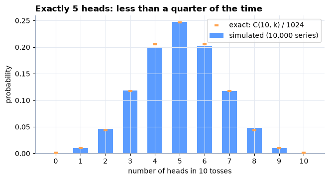
2.1 Simulate 10,000 series of 10 tosses (an array of shape (10_000, 10)), count the heads in each series and
estimate the probability of getting exactly 5 heads. Compare with the exact value
(math.comb(10, 5) / 2**10).
rng = np.random.default_rng(10)
# TO COMPLETE: n_heads = number of heads in each of the 10,000 series; p5 = proportion of series with 5 heads
n_heads = None
p5 = None
p5_exact = math.comb(10, 5) / 2**10
check("P(5 heads in 10), simulated", p5, p5_exact, 0.015)

if ready(n_heads):
    k = np.arange(11)
    exact = np.array([math.comb(10, j) for j in k]) / 2**10
    simulated = np.bincount(n_heads, minlength=11) / len(n_heads)
    fig, ax = plt.subplots()
    ax.bar(k, simulated, width=0.6, color=BLUE, label="simulated (10,000 series)")
    ax.scatter(k, exact, color=ORANGE, zorder=3, s=40, marker="_", linewidths=3, label="exact: C(10, k) / 1024")
    ax.set_xticks(k)
    ax.set_xlabel("number of heads in 10 tosses")
    ax.set_ylabel("probability")
    ax.set_title("Exactly 5 heads: less than a quarter of the time")
    ax.legend()
    plt.show()
Show the solution
rng = np.random.default_rng(10)
# TO COMPLETE: n_heads = number of heads in each of the 10,000 series; p5 = proportion of series with 5 heads
series = rng.random((10_000, 10)) < 0.5
n_heads = series.sum(axis=1)
p5 = np.mean(n_heads == 5)
p5_exact = math.comb(10, 5) / 2**10
check("P(5 heads in 10), simulated", p5, p5_exact, 0.015)

if ready(n_heads):
    k = np.arange(11)
    exact = np.array([math.comb(10, j) for j in k]) / 2**10
    simulated = np.bincount(n_heads, minlength=11) / len(n_heads)
    fig, ax = plt.subplots()
    ax.bar(k, simulated, width=0.6, color=BLUE, label="simulated (10,000 series)")
    ax.scatter(k, exact, color=ORANGE, zorder=3, s=40, marker="_", linewidths=3, label="exact: C(10, k) / 1024")
    ax.set_xticks(k)
    ax.set_xlabel("number of heads in 10 tosses")
    ax.set_ylabel("probability")
    ax.set_title("Exactly 5 heads: less than a quarter of the time")
    ax.legend()
    plt.show()
✓ P(5 heads in 10), simulated = 0.247 (expected ≈ 0.246094)
rng = np.random.default_rng(10)
# TO COMPLETE: n_heads = number of heads in each of the 10,000 series; p5 = proportion of series with 5 heads
series = rng.random((10_000, 10)) < 0.5
n_heads = series.sum(axis=1)
p5 = np.mean(n_heads == 5)
p5_exact = math.comb(10, 5) / 2**10
check("P(5 heads in 10), simulated", p5, p5_exact, 0.015)

if ready(n_heads):
    k = np.arange(11)
    exact = np.array([math.comb(10, j) for j in k]) / 2**10
    simulated = np.bincount(n_heads, minlength=11) / len(n_heads)
    fig, ax = plt.subplots()
    ax.bar(k, simulated, width=0.6, color=BLUE, label="simulated (10,000 series)")
    ax.scatter(k, exact, color=ORANGE, zorder=3, s=40, marker="_", linewidths=3, label="exact: C(10, k) / 1024")
    ax.set_xticks(k)
    ax.set_xlabel("number of heads in 10 tosses")
    ax.set_ylabel("probability")
    ax.set_title("Exactly 5 heads: less than a quarter of the time")
    ax.legend()
    plt.show()
✓ P(5 heads in 10), simulated = 0.247 (expected ≈ 0.246094)
Exactly five heads happens in only 24.6% of cases (252 sequences out of 1,024): six heads and four tails, or the reverse, happens 41% of the time. A coin that gives 6 and 4 is not cheating. See the film of session 1, chapter “A probability is a proportion”.
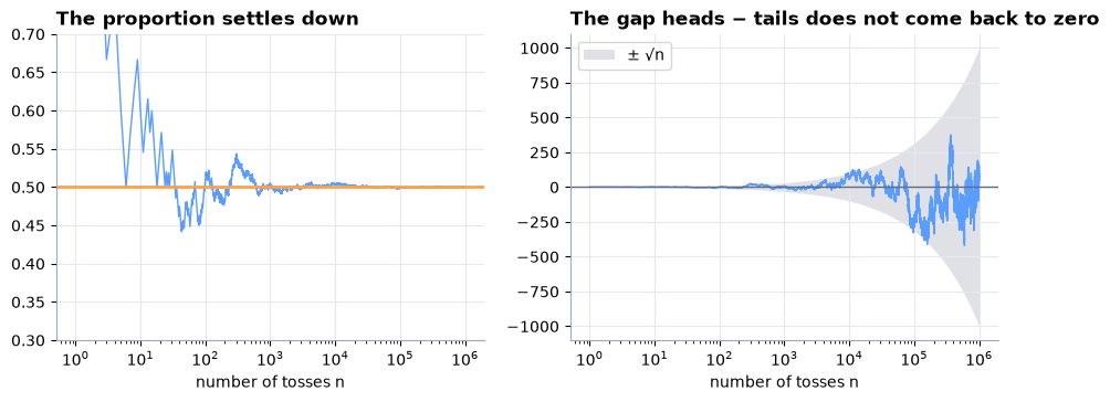
2.2 Toss the coin a million times. After each toss , compute the proportion of heads
and the gap between heads and tails (hint: np.cumsum). Plot both
curves as functions of (logarithmic horizontal axis), with the orange line for the proportion and the
grey band for the gap.
Predict. Does the gap heads − tails come back towards zero as grows?
2.2 Toss the coin a million times. After each toss , compute the proportion of heads
and the gap between heads and tails (hint: np.cumsum). Plot both
curves as functions of (logarithmic horizontal axis), with the orange line for the proportion and the
grey band for the gap.
Predict. Does the gap heads − tails come back towards zero as grows?
rng = np.random.default_rng(2)
n = np.arange(1, 1_000_001)
# TO COMPLETE: proportion[i] = proportion of heads after i+1 tosses; gap[i] = heads − tails after i+1 tosses
proportion = None
gap = None

if ready(proportion, gap):
    print(f"after 10,000 tosses: {proportion[9_999]:.4%}; after a million: {proportion[-1]:.4%}")
    print(f"gap heads − tails after a million tosses: {gap[-1]:+d}")
    fig, (a1, a2) = plt.subplots(1, 2, figsize=(11, 3.6))
    a1.semilogx(n, proportion, color=BLUE, lw=1)
    a1.axhline(0.5, color=ORANGE, lw=2)
    a1.set_ylim(0.3, 0.7)
    a1.set_title("The proportion settles down")
    a1.set_xlabel("number of tosses n")
    a2.semilogx(n, gap, color=BLUE, lw=1)
    a2.fill_between(n, -np.sqrt(n), np.sqrt(n), color=GREY, alpha=0.2, lw=0, label="± √n")
    a2.axhline(0, color=GREY, lw=1)
    a2.set_title("The gap heads − tails does not come back to zero")
    a2.set_xlabel("number of tosses n")
    a2.legend(loc="upper left")
    plt.show()
Show the solution
rng = np.random.default_rng(2)
n = np.arange(1, 1_000_001)
# TO COMPLETE: proportion[i] = proportion of heads after i+1 tosses; gap[i] = heads − tails after i+1 tosses
x = tosses(1_000_000, rng)
k = np.cumsum(x)
proportion = k / n
gap = 2 * k - n

if ready(proportion, gap):
    print(f"after 10,000 tosses: {proportion[9_999]:.4%}; after a million: {proportion[-1]:.4%}")
    print(f"gap heads − tails after a million tosses: {gap[-1]:+d}")
    fig, (a1, a2) = plt.subplots(1, 2, figsize=(11, 3.6))
    a1.semilogx(n, proportion, color=BLUE, lw=1)
    a1.axhline(0.5, color=ORANGE, lw=2)
    a1.set_ylim(0.3, 0.7)
    a1.set_title("The proportion settles down")
    a1.set_xlabel("number of tosses n")
    a2.semilogx(n, gap, color=BLUE, lw=1)
    a2.fill_between(n, -np.sqrt(n), np.sqrt(n), color=GREY, alpha=0.2, lw=0, label="± √n")
    a2.axhline(0, color=GREY, lw=1)
    a2.set_title("The gap heads − tails does not come back to zero")
    a2.set_xlabel("number of tosses n")
    a2.legend(loc="upper left")
    plt.show()
after 10,000 tosses: 50.2800%; after a million: 50.0047% gap heads − tails after a million tosses: +94
rng = np.random.default_rng(2)
n = np.arange(1, 1_000_001)
# TO COMPLETE: proportion[i] = proportion of heads after i+1 tosses; gap[i] = heads − tails after i+1 tosses
x = tosses(1_000_000, rng)
k = np.cumsum(x)
proportion = k / n
gap = 2 * k - n

if ready(proportion, gap):
    print(f"after 10,000 tosses: {proportion[9_999]:.4%}; after a million: {proportion[-1]:.4%}")
    print(f"gap heads − tails after a million tosses: {gap[-1]:+d}")
    fig, (a1, a2) = plt.subplots(1, 2, figsize=(11, 3.6))
    a1.semilogx(n, proportion, color=BLUE, lw=1)
    a1.axhline(0.5, color=ORANGE, lw=2)
    a1.set_ylim(0.3, 0.7)
    a1.set_title("The proportion settles down")
    a1.set_xlabel("number of tosses n")
    a2.semilogx(n, gap, color=BLUE, lw=1)
    a2.fill_between(n, -np.sqrt(n), np.sqrt(n), color=GREY, alpha=0.2, lw=0, label="± √n")
    a2.axhline(0, color=GREY, lw=1)
    a2.set_title("The gap heads − tails does not come back to zero")
    a2.set_xlabel("number of tosses n")
    a2.legend(loc="upper left")
    plt.show()
after 10,000 tosses: 50.2800%; after a million: 50.0047% gap heads − tails after a million tosses: +94
The gap wanders and typically grows like (it stays in the grey band most of the time); it does not come back to zero. But : divided by , it shrinks to nothing, and the proportion tends to 1/2. Chance does not even out: it gets diluted. This is exactly the law of large numbers, and it is also the refutation of the “gambler's fallacy” (after a run of tails, heads is not “due”).
3. π with darts (20 min)
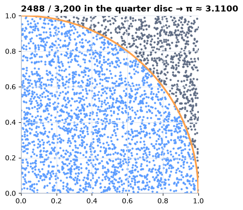
We throw uniform points into the square . The proportion of points that land in the quarter disc estimates its area, ; so proportion estimates .
3.1 Write estimate_pi(n, rng), then draw 3,200 darts: in blue those in the quarter disc, in grey the others,
and the arc in orange.
3. π with darts (20 min)
We throw uniform points into the square . The proportion of points that land in the quarter disc estimates its area, ; so proportion estimates .
3.1 Write estimate_pi(n, rng), then draw 3,200 darts: in blue those in the quarter disc, in grey the others,
and the arc in orange.
def estimate_pi(n, rng):
    """Estimate of π from n uniform darts in the unit square."""
    # TO COMPLETE
    return None


check("estimate_pi(1_000_000)", estimate_pi(1_000_000, np.random.default_rng(21)), math.pi, 0.01)

rng = np.random.default_rng(21)
x, y = rng.random(3200), rng.random(3200)
inside = x * x + y * y <= 1
t = np.linspace(0, math.pi / 2, 300)
fig, ax = plt.subplots(figsize=(4.6, 4.6))
ax.scatter(x[inside], y[inside], s=4, color=BLUE)
ax.scatter(x[~inside], y[~inside], s=4, color=GREY)
ax.plot(np.cos(t), np.sin(t), color=ORANGE, lw=2.5)
ax.set_aspect("equal")
ax.set_xlim(0, 1)
ax.set_ylim(0, 1)
ax.set_title(f"{inside.sum()} / 3,200 in the quarter disc → π ≈ {4 * inside.mean():.4f}")
plt.show()
Show the solution
def estimate_pi(n, rng):
    """Estimate of π from n uniform darts in the unit square."""
    # TO COMPLETE
    x, y = rng.random(n), rng.random(n)
    return 4 * np.mean(x * x + y * y <= 1)


check("estimate_pi(1_000_000)", estimate_pi(1_000_000, np.random.default_rng(21)), math.pi, 0.01)

rng = np.random.default_rng(21)
x, y = rng.random(3200), rng.random(3200)
inside = x * x + y * y <= 1
t = np.linspace(0, math.pi / 2, 300)
fig, ax = plt.subplots(figsize=(4.6, 4.6))
ax.scatter(x[inside], y[inside], s=4, color=BLUE)
ax.scatter(x[~inside], y[~inside], s=4, color=GREY)
ax.plot(np.cos(t), np.sin(t), color=ORANGE, lw=2.5)
ax.set_aspect("equal")
ax.set_xlim(0, 1)
ax.set_ylim(0, 1)
ax.set_title(f"{inside.sum()} / 3,200 in the quarter disc → π ≈ {4 * inside.mean():.4f}")
plt.show()
✓ estimate_pi(1_000_000) = 3.14069 (expected ≈ 3.14159)
def estimate_pi(n, rng):
    """Estimate of π from n uniform darts in the unit square."""
    # TO COMPLETE
    x, y = rng.random(n), rng.random(n)
    return 4 * np.mean(x * x + y * y <= 1)


check("estimate_pi(1_000_000)", estimate_pi(1_000_000, np.random.default_rng(21)), math.pi, 0.01)

rng = np.random.default_rng(21)
x, y = rng.random(3200), rng.random(3200)
inside = x * x + y * y <= 1
t = np.linspace(0, math.pi / 2, 300)
fig, ax = plt.subplots(figsize=(4.6, 4.6))
ax.scatter(x[inside], y[inside], s=4, color=BLUE)
ax.scatter(x[~inside], y[~inside], s=4, color=GREY)
ax.plot(np.cos(t), np.sin(t), color=ORANGE, lw=2.5)
ax.set_aspect("equal")
ax.set_xlim(0, 1)
ax.set_ylim(0, 1)
ax.set_title(f"{inside.sum()} / 3,200 in the quarter disc → π ≈ {4 * inside.mean():.4f}")
plt.show()
✓ estimate_pi(1_000_000) = 3.14069 (expected ≈ 3.14159)
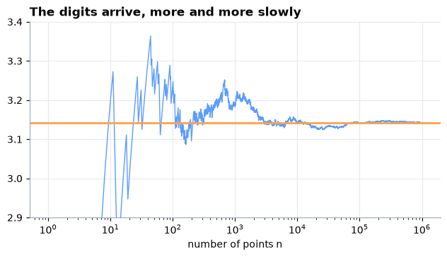
3.2 Follow the estimate as the number of points grows up to a million (hint: the cumulative mean of the
indicator inside). Plot it (logarithmic horizontal axis) with the orange line .
rng = np.random.default_rng(1812)
N = 1_000_000
n = np.arange(1, N + 1)
# TO COMPLETE: estimate[i] = estimate of π with the first i+1 points
estimate = None

if ready(estimate):
    for m in (100, 10_000, 1_000_000):
        print(f"n = {m:>9,}: π ≈ {estimate[m - 1]:.5f}   (error {estimate[m - 1] - math.pi:+.5f})")
    fig, ax = plt.subplots()
    ax.semilogx(n, estimate, color=BLUE, lw=1)
    ax.axhline(math.pi, color=ORANGE, lw=2)
    ax.set_ylim(2.9, 3.4)
    ax.set_xlabel("number of points n")
    ax.set_title("The digits arrive, more and more slowly")
    plt.show()
Show the solution
rng = np.random.default_rng(1812)
N = 1_000_000
n = np.arange(1, N + 1)
# TO COMPLETE: estimate[i] = estimate of π with the first i+1 points
x, y = rng.random(N), rng.random(N)
estimate = 4 * np.cumsum(x * x + y * y <= 1) / n

if ready(estimate):
    for m in (100, 10_000, 1_000_000):
        print(f"n = {m:>9,}: π ≈ {estimate[m - 1]:.5f}   (error {estimate[m - 1] - math.pi:+.5f})")
    fig, ax = plt.subplots()
    ax.semilogx(n, estimate, color=BLUE, lw=1)
    ax.axhline(math.pi, color=ORANGE, lw=2)
    ax.set_ylim(2.9, 3.4)
    ax.set_xlabel("number of points n")
    ax.set_title("The digits arrive, more and more slowly")
    plt.show()
n = 100: π ≈ 3.24000 (error +0.09841) n = 10,000: π ≈ 3.14200 (error +0.00041) n = 1,000,000: π ≈ 3.14190 (error +0.00031)
rng = np.random.default_rng(1812)
N = 1_000_000
n = np.arange(1, N + 1)
# TO COMPLETE: estimate[i] = estimate of π with the first i+1 points
x, y = rng.random(N), rng.random(N)
estimate = 4 * np.cumsum(x * x + y * y <= 1) / n

if ready(estimate):
    for m in (100, 10_000, 1_000_000):
        print(f"n = {m:>9,}: π ≈ {estimate[m - 1]:.5f}   (error {estimate[m - 1] - math.pi:+.5f})")
    fig, ax = plt.subplots()
    ax.semilogx(n, estimate, color=BLUE, lw=1)
    ax.axhline(math.pi, color=ORANGE, lw=2)
    ax.set_ylim(2.9, 3.4)
    ax.set_xlabel("number of points n")
    ax.set_title("The digits arrive, more and more slowly")
    plt.show()
n = 100: π ≈ 3.24000 (error +0.09841) n = 10,000: π ≈ 3.14200 (error +0.00041) n = 1,000,000: π ≈ 3.14190 (error +0.00031)
4. The bell curve narrows (25 min)
The estimate of π is itself drawn at random: redo the experiment and you get another number. To measure its error, we repeat it times and look at the shape of the results.
Predict. If we take four times as many points, does the bell curve of the estimates become four times narrower? Twice? Sixteen times?
4.1 Write repeat(n, R, rng), which returns an array of independent estimates of π, each with
points (a loop over is enough).
def repeat(n, R, rng):
    """R independent estimates of π, each with n points."""
    # TO COMPLETE
    return None


rng = np.random.default_rng(1812)
sizes = [100, 400, 1600, 6400]
bells = {n: repeat(n, 2000, rng) for n in sizes}
if ready(*bells.values()):
    fig, ax = plt.subplots()
    shades = ["#C9DCFF", "#9DC0FF", "#78A9FF", BLUE]
    for n, c in zip(sizes, shades):
        ax.hist(bells[n], bins=np.linspace(2.6, 3.7, 89), color=c, alpha=0.9, label=f"n = {n}")
    ax.axvline(math.pi, color=ORANGE, lw=2)
    ax.set_xlabel("estimate of π")
    ax.set_title("× 4 points: the bell curve narrows")
    ax.legend()
    plt.show()
    for n in sizes:
        print(f"n = {n:>5}: standard deviation of the 2,000 estimates = {bells[n].std(ddof=1):.4f}")
Show the solution
def repeat(n, R, rng):
    """R independent estimates of π, each with n points."""
    # TO COMPLETE
    return np.array([estimate_pi(n, rng) for _ in range(R)])


rng = np.random.default_rng(1812)
sizes = [100, 400, 1600, 6400]
bells = {n: repeat(n, 2000, rng) for n in sizes}
if ready(*bells.values()):
    fig, ax = plt.subplots()
    shades = ["#C9DCFF", "#9DC0FF", "#78A9FF", BLUE]
    for n, c in zip(sizes, shades):
        ax.hist(bells[n], bins=np.linspace(2.6, 3.7, 89), color=c, alpha=0.9, label=f"n = {n}")
    ax.axvline(math.pi, color=ORANGE, lw=2)
    ax.set_xlabel("estimate of π")
    ax.set_title("× 4 points: the bell curve narrows")
    ax.legend()
    plt.show()
    for n in sizes:
        print(f"n = {n:>5}: standard deviation of the 2,000 estimates = {bells[n].std(ddof=1):.4f}")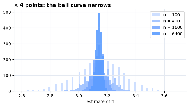
n =   100: standard deviation of the 2,000 estimates = 0.1676
n =   400: standard deviation of the 2,000 estimates = 0.0847
n =  1600: standard deviation of the 2,000 estimates = 0.0411
n =  6400: standard deviation of the 2,000 estimates = 0.0205
def repeat(n, R, rng):
    """R independent estimates of π, each with n points."""
    # TO COMPLETE
    return np.array([estimate_pi(n, rng) for _ in range(R)])


rng = np.random.default_rng(1812)
sizes = [100, 400, 1600, 6400]
bells = {n: repeat(n, 2000, rng) for n in sizes}
if ready(*bells.values()):
    fig, ax = plt.subplots()
    shades = ["#C9DCFF", "#9DC0FF", "#78A9FF", BLUE]
    for n, c in zip(sizes, shades):
        ax.hist(bells[n], bins=np.linspace(2.6, 3.7, 89), color=c, alpha=0.9, label=f"n = {n}")
    ax.axvline(math.pi, color=ORANGE, lw=2)
    ax.set_xlabel("estimate of π")
    ax.set_title("× 4 points: the bell curve narrows")
    ax.legend()
    plt.show()
    for n in sizes:
        print(f"n = {n:>5}: standard deviation of the 2,000 estimates = {bells[n].std(ddof=1):.4f}")
n = 100: standard deviation of the 2,000 estimates = 0.1676 n = 400: standard deviation of the 2,000 estimates = 0.0847 n = 1600: standard deviation of the 2,000 estimates = 0.0411 n = 6400: standard deviation of the 2,000 estimates = 0.0205
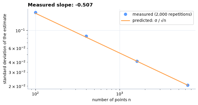
4.2 Plot the standard deviation of the estimates as a function of on a log-log scale and measure the slope
by a regression (np.polyfit(np.log(n), np.log(std_dev), 1)). Compare with the prediction with
and : this is the standard deviation of one dart (multiplied by 4).
sigma = 4 * math.sqrt(math.pi / 4 * (1 - math.pi / 4))
print(f"σ of one dart: {sigma:.4f}")
# TO COMPLETE: std_devs = array of the measured standard deviations; slope = slope of the log-log line
nn = np.array(sizes)
std_devs = None
slope = None
check("log-log slope", slope, -0.5, 0.05)

if ready(std_devs):
    fig, ax = plt.subplots()
    ax.loglog(nn, std_devs, "o", color=BLUE, ms=7, label="measured (2,000 repetitions)")
    ax.loglog(nn, sigma / np.sqrt(nn), color=ORANGE, lw=2, label="predicted: σ / √n")
    ax.set_xlabel("number of points n")
    ax.set_ylabel("standard deviation of the estimate")
    ax.set_title(f"Measured slope: {slope:.3f}")
    ax.legend()
    plt.show()
Show the solution
sigma = 4 * math.sqrt(math.pi / 4 * (1 - math.pi / 4))
print(f"σ of one dart: {sigma:.4f}")
# TO COMPLETE: std_devs = array of the measured standard deviations; slope = slope of the log-log line
nn = np.array(sizes)
std_devs = np.array([bells[n].std(ddof=1) for n in sizes])
slope, intercept = np.polyfit(np.log(nn), np.log(std_devs), 1)
check("log-log slope", slope, -0.5, 0.05)

if ready(std_devs):
    fig, ax = plt.subplots()
    ax.loglog(nn, std_devs, "o", color=BLUE, ms=7, label="measured (2,000 repetitions)")
    ax.loglog(nn, sigma / np.sqrt(nn), color=ORANGE, lw=2, label="predicted: σ / √n")
    ax.set_xlabel("number of points n")
    ax.set_ylabel("standard deviation of the estimate")
    ax.set_title(f"Measured slope: {slope:.3f}")
    ax.legend()
    plt.show()
σ of one dart: 1.6422
✓ log-log slope = -0.50678 (expected ≈ -0.5)
sigma = 4 * math.sqrt(math.pi / 4 * (1 - math.pi / 4))
print(f"σ of one dart: {sigma:.4f}")
# TO COMPLETE: std_devs = array of the measured standard deviations; slope = slope of the log-log line
nn = np.array(sizes)
std_devs = np.array([bells[n].std(ddof=1) for n in sizes])
slope, intercept = np.polyfit(np.log(nn), np.log(std_devs), 1)
check("log-log slope", slope, -0.5, 0.05)

if ready(std_devs):
    fig, ax = plt.subplots()
    ax.loglog(nn, std_devs, "o", color=BLUE, ms=7, label="measured (2,000 repetitions)")
    ax.loglog(nn, sigma / np.sqrt(nn), color=ORANGE, lw=2, label="predicted: σ / √n")
    ax.set_xlabel("number of points n")
    ax.set_ylabel("standard deviation of the estimate")
    ax.set_title(f"Measured slope: {slope:.3f}")
    ax.legend()
    plt.show()
σ of one dart: 1.6422
✓ log-log slope = -0.50678 (expected ≈ -0.5)
The slope is −1/2, up to fluctuations: the error decreases like . Four times as many points divide the error by two; a hundred times as many points give one more digit. The bell shape is the one predicted by the central limit theorem. See the film of session 1, chapter “How many samples?”.
5. Proving that we are right: the confidence interval (20 min)
For a mean of samples with variance , the central limit theorem gives the asymptotic 95% confidence interval: estimate , where is the sample standard deviation of the draws.
5.1 Write ci95(samples), which returns the pair (estimate, half-width) from the array of individual samples
(for π, the samples are the values ).
5. Proving that we are right: the confidence interval (20 min)
For a mean of samples with variance , the central limit theorem gives the asymptotic 95% confidence interval: estimate , where is the sample standard deviation of the draws.
5.1 Write ci95(samples), which returns the pair (estimate, half-width) from the array of individual samples
(for π, the samples are the values ).
def ci95(samples):
    """Mean and half-width of the asymptotic 95% confidence interval."""
    # TO COMPLETE
    return None, None


rng = np.random.default_rng(21)
x, y = rng.random(1_000_000), rng.random(1_000_000)
est, half = ci95(4.0 * (x * x + y * y <= 1))
if ready(est, half):
    print(f"π ≈ {est:.4f} ± {half:.4f}   (is π = {math.pi:.4f} inside? {abs(est - math.pi) <= half})")
check("half-width with a million points", half, 1.96 * sigma / 1000, 0.0002)
Show the solution
def ci95(samples):
    """Mean and half-width of the asymptotic 95% confidence interval."""
    # TO COMPLETE
    samples = np.asarray(samples, dtype=float)
    return samples.mean(), 1.96 * samples.std(ddof=1) / math.sqrt(len(samples))


rng = np.random.default_rng(21)
x, y = rng.random(1_000_000), rng.random(1_000_000)
est, half = ci95(4.0 * (x * x + y * y <= 1))
if ready(est, half):
    print(f"π ≈ {est:.4f} ± {half:.4f}   (is π = {math.pi:.4f} inside? {abs(est - math.pi) <= half})")
check("half-width with a million points", half, 1.96 * sigma / 1000, 0.0002)
π ≈ 3.1407 ± 0.0032 (is π = 3.1416 inside? True) ✓ half-width with a million points = 0.00321991 (expected ≈ 0.00321868)
def ci95(samples):
    """Mean and half-width of the asymptotic 95% confidence interval."""
    # TO COMPLETE
    samples = np.asarray(samples, dtype=float)
    return samples.mean(), 1.96 * samples.std(ddof=1) / math.sqrt(len(samples))


rng = np.random.default_rng(21)
x, y = rng.random(1_000_000), rng.random(1_000_000)
est, half = ci95(4.0 * (x * x + y * y <= 1))
if ready(est, half):
    print(f"π ≈ {est:.4f} ± {half:.4f}   (is π = {math.pi:.4f} inside? {abs(est - math.pi) <= half})")
check("half-width with a million points", half, 1.96 * sigma / 1000, 0.0002)
π ≈ 3.1407 ± 0.0032 (is π = 3.1416 inside? True) ✓ half-width with a million points = 0.00321991 (expected ≈ 0.00321868)
5.2 Build 100 confidence intervals for π, each with points, and draw them stacked: in blue those that contain π, in red those that miss it, and the vertical orange line .
Predict. How many of the hundred intervals should miss π?
rng = np.random.default_rng(1812)
# TO COMPLETE: centres[i], halves[i] = estimate and half-width of the i-th interval
centres, halves = None, None

if ready(centres, halves):
    hit = np.abs(centres - math.pi) <= halves
    fig, ax = plt.subplots(figsize=(6.5, 7))
    for i in range(100):
        colour = BLUE if hit[i] else RED
        ax.plot([centres[i] - halves[i], centres[i] + halves[i]], [i, i], color=colour, lw=1.6)
        ax.plot(centres[i], i, "o", color=colour, ms=2.5)
    ax.axvline(math.pi, color=ORANGE, lw=2)
    ax.set_yticks([])
    ax.set_xlabel("95% confidence interval (N = 1,000 points)")
    ax.set_title(f"{hit.sum()} intervals out of 100 catch π")
    plt.show()
Show the solution
rng = np.random.default_rng(1812)
# TO COMPLETE: centres[i], halves[i] = estimate and half-width of the i-th interval
centres, halves = np.zeros(100), np.zeros(100)
for i in range(100):
    x, y = rng.random(1000), rng.random(1000)
    centres[i], halves[i] = ci95(4.0 * (x * x + y * y <= 1))

if ready(centres, halves):
    hit = np.abs(centres - math.pi) <= halves
    fig, ax = plt.subplots(figsize=(6.5, 7))
    for i in range(100):
        colour = BLUE if hit[i] else RED
        ax.plot([centres[i] - halves[i], centres[i] + halves[i]], [i, i], color=colour, lw=1.6)
        ax.plot(centres[i], i, "o", color=colour, ms=2.5)
    ax.axvline(math.pi, color=ORANGE, lw=2)
    ax.set_yticks([])
    ax.set_xlabel("95% confidence interval (N = 1,000 points)")
    ax.set_title(f"{hit.sum()} intervals out of 100 catch π")
    plt.show()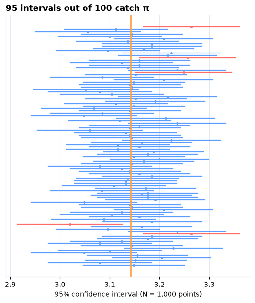
rng = np.random.default_rng(1812)
# TO COMPLETE: centres[i], halves[i] = estimate and half-width of the i-th interval
centres, halves = np.zeros(100), np.zeros(100)
for i in range(100):
    x, y = rng.random(1000), rng.random(1000)
    centres[i], halves[i] = ci95(4.0 * (x * x + y * y <= 1))

if ready(centres, halves):
    hit = np.abs(centres - math.pi) <= halves
    fig, ax = plt.subplots(figsize=(6.5, 7))
    for i in range(100):
        colour = BLUE if hit[i] else RED
        ax.plot([centres[i] - halves[i], centres[i] + halves[i]], [i, i], color=colour, lw=1.6)
        ax.plot(centres[i], i, "o", color=colour, ms=2.5)
    ax.axvline(math.pi, color=ORANGE, lw=2)
    ax.set_yticks([])
    ax.set_xlabel("95% confidence interval (N = 1,000 points)")
    ax.set_title(f"{hit.sum()} intervals out of 100 catch π")
    plt.show()
5.3 Measure the coverage rate over 2,000 intervals (still ): the proportion of those that contain π. Is it compatible with 95%? (The standard deviation of a proportion estimated from 2,000 trials is about .)
rng = np.random.default_rng(7)
# TO COMPLETE: coverage = proportion of the 2,000 intervals that contain π
coverage = None
check("coverage rate", coverage, 0.95, 0.015)
Show the solution
rng = np.random.default_rng(7)
# TO COMPLETE: coverage = proportion of the 2,000 intervals that contain π
x, y = rng.random((2000, 1000)), rng.random((2000, 1000))
t = 4.0 * (x * x + y * y <= 1)
m = t.mean(axis=1)
h = 1.96 * t.std(axis=1, ddof=1) / math.sqrt(1000)
coverage = np.mean(np.abs(m - math.pi) <= h)
check("coverage rate", coverage, 0.95, 0.015)
✓ coverage rate = 0.953 (expected ≈ 0.95)
rng = np.random.default_rng(7)
# TO COMPLETE: coverage = proportion of the 2,000 intervals that contain π
x, y = rng.random((2000, 1000)), rng.random((2000, 1000))
t = 4.0 * (x * x + y * y <= 1)
m = t.mean(axis=1)
h = 1.96 * t.std(axis=1, ddof=1) / math.sqrt(1000)
coverage = np.mean(np.abs(m - math.pi) <= h)
check("coverage rate", coverage, 0.95, 0.015)
✓ coverage rate = 0.953 (expected ≈ 0.95)
The measured rate is close to 95% (to within about ± 0.01). Correct interpretation: the 95% describes the method (over a large number of repetitions, 95% of the intervals built this way contain π), not a particular interval: once computed, an interval either contains π or does not. A wrong sentence to avoid: “π has a 95% chance of being in [3.10, 3.18]”.
5.4 The answer to Ulam. How many games of solitaire must be played to know the probability of success to within ± 1% (half-width of the 95% interval), whatever ? Hint: the variance of an indicator is . Then check by simulation, with (the worst case), that the half-width obtained is indeed about 0.01.
5.4 The answer to Ulam. How many games of solitaire must be played to know the probability of success to within ± 1% (half-width of the 95% interval), whatever ? Hint: the variance of an indicator is . Then check by simulation, with (the worst case), that the half-width obtained is indeed about 0.01.
# TO COMPLETE: n_ulam = number of games needed (an integer)
n_ulam = None
check("games needed for ± 1%", n_ulam, 9604, 0.5)
Show the solution
# TO COMPLETE: n_ulam = number of games needed (an integer)
n_ulam = math.ceil((1.96 * 0.5 / 0.01) ** 2)
games = (np.random.default_rng(1946).random(n_ulam) < 0.5).astype(float)
print("half-width obtained:", round(ci95(games)[1], 4))
check("games needed for ± 1%", n_ulam, 9604, 0.5)
half-width obtained: 0.01 ✓ games needed for ± 1% = 9604 (expected ≈ 9604)
# TO COMPLETE: n_ulam = number of games needed (an integer)
n_ulam = math.ceil((1.96 * 0.5 / 0.01) ** 2)
games = (np.random.default_rng(1946).random(n_ulam) < 0.5).astype(float)
print("half-width obtained:", round(ci95(games)[1], 4))
check("games needed for ± 1%", n_ulam, 9604, 0.5)
half-width obtained: 0.01 ✓ games needed for ± 1% = 9604 (expected ≈ 9604)
6. Application: the price of a call option (15 min)
A European call option with strike and maturity pays . In the Black–Scholes model, under the “risk-neutral” probability, with , and the price is . The judge is the Black–Scholes formula, given below.
6.1 Estimate the price with samples for , , , , give the 95% confidence interval and check that it contains the exact price.
def phi(x):
    """Cumulative distribution function of the standard normal distribution."""
    return 0.5 * (1 + math.erf(x / math.sqrt(2)))


def bs_call(S0, K, r, sigma, T):
    """The judge: Black–Scholes price of a European call option."""
    d1 = (math.log(S0 / K) + (r + sigma**2 / 2) * T) / (sigma * math.sqrt(T))
    return S0 * phi(d1) - K * math.exp(-r * T) * phi(d1 - sigma * math.sqrt(T))


S0, K, r, sig, T = 100.0, 100.0, 0.05, 0.20, 1.0
judge = bs_call(S0, K, r, sig, T)
rng = np.random.default_rng(1973)
# TO COMPLETE: payoffs = discounted payoffs e^{-rT} (S_T − K)^+ for 100,000 samples
payoffs = None
if ready(payoffs):
    price, half = ci95(payoffs)
    print(f"Monte Carlo: {price:.3f} ± {half:.3f}   |   Black–Scholes: {judge:.4f}   |   inside: {abs(price - judge) <= half}")
    check("price of the call option", price, judge, 0.15)
Show the solution
def phi(x):
    """Cumulative distribution function of the standard normal distribution."""
    return 0.5 * (1 + math.erf(x / math.sqrt(2)))


def bs_call(S0, K, r, sigma, T):
    """The judge: Black–Scholes price of a European call option."""
    d1 = (math.log(S0 / K) + (r + sigma**2 / 2) * T) / (sigma * math.sqrt(T))
    return S0 * phi(d1) - K * math.exp(-r * T) * phi(d1 - sigma * math.sqrt(T))


S0, K, r, sig, T = 100.0, 100.0, 0.05, 0.20, 1.0
judge = bs_call(S0, K, r, sig, T)
rng = np.random.default_rng(1973)
# TO COMPLETE: payoffs = discounted payoffs e^{-rT} (S_T − K)^+ for 100,000 samples
Z = rng.standard_normal(100_000)
ST = S0 * np.exp((r - sig**2 / 2) * T + sig * math.sqrt(T) * Z)
payoffs = math.exp(-r * T) * np.maximum(ST - K, 0)
if ready(payoffs):
    price, half = ci95(payoffs)
    print(f"Monte Carlo: {price:.3f} ± {half:.3f}   |   Black–Scholes: {judge:.4f}   |   inside: {abs(price - judge) <= half}")
    check("price of the call option", price, judge, 0.15)
Monte Carlo: 10.427 ± 0.091 | Black–Scholes: 10.4506 | inside: True ✓ price of the call option = 10.4265 (expected ≈ 10.4506)
def phi(x):
    """Cumulative distribution function of the standard normal distribution."""
    return 0.5 * (1 + math.erf(x / math.sqrt(2)))


def bs_call(S0, K, r, sigma, T):
    """The judge: Black–Scholes price of a European call option."""
    d1 = (math.log(S0 / K) + (r + sigma**2 / 2) * T) / (sigma * math.sqrt(T))
    return S0 * phi(d1) - K * math.exp(-r * T) * phi(d1 - sigma * math.sqrt(T))


S0, K, r, sig, T = 100.0, 100.0, 0.05, 0.20, 1.0
judge = bs_call(S0, K, r, sig, T)
rng = np.random.default_rng(1973)
# TO COMPLETE: payoffs = discounted payoffs e^{-rT} (S_T − K)^+ for 100,000 samples
Z = rng.standard_normal(100_000)
ST = S0 * np.exp((r - sig**2 / 2) * T + sig * math.sqrt(T) * Z)
payoffs = math.exp(-r * T) * np.maximum(ST - K, 0)
if ready(payoffs):
    price, half = ci95(payoffs)
    print(f"Monte Carlo: {price:.3f} ± {half:.3f}   |   Black–Scholes: {judge:.4f}   |   inside: {abs(price - judge) <= half}")
    check("price of the call option", price, judge, 0.15)
Monte Carlo: 10.427 ± 0.091 | Black–Scholes: 10.4506 | inside: True ✓ price of the call option = 10.4265 (expected ≈ 10.4506)
6.2 How many samples would be needed for a half-width of one cent? Predict with (the standard deviation of the payoffs), then check with the number obtained.
# TO COMPLETE: n_cent = predicted number of samples for a half-width of €0.01
n_cent = None
check("samples for ± 1 cent", n_cent, 8.4e6, 0.4e6)
Show the solution
# TO COMPLETE: n_cent = predicted number of samples for a half-width of €0.01
n_cent = math.ceil((1.96 * payoffs.std(ddof=1) / 0.01) ** 2)
print(f"samples needed: {n_cent:,}")
Z = np.random.default_rng(1974).standard_normal(n_cent)
g = math.exp(-r * T) * np.maximum(S0 * np.exp((r - sig**2 / 2) * T + sig * math.sqrt(T) * Z) - K, 0)
print("half-width obtained: %.4f" % ci95(g)[1])
check("samples for ± 1 cent", n_cent, 8.4e6, 0.4e6)
samples needed: 8,256,475
half-width obtained: 0.0100
✓ samples for ± 1 cent = 8.25648e+06 (expected ≈ 8.4e+06)
# TO COMPLETE: n_cent = predicted number of samples for a half-width of €0.01
n_cent = math.ceil((1.96 * payoffs.std(ddof=1) / 0.01) ** 2)
print(f"samples needed: {n_cent:,}")
Z = np.random.default_rng(1974).standard_normal(n_cent)
g = math.exp(-r * T) * np.maximum(S0 * np.exp((r - sig**2 / 2) * T + sig * math.sqrt(T) * Z) - K, 0)
print("half-width obtained: %.4f" % ci95(g)[1])
check("samples for ± 1 cent", n_cent, 8.4e6, 0.4e6)
samples needed: 8,256,475
half-width obtained: 0.0100
✓ samples for ± 1 cent = 8.25648e+06 (expected ≈ 8.4e+06)
euros, so we need million samples. Dividing the error by 10 costs 100 times more samples: that is the price of one digit. Session 2 shows how to divide the error without paying this price.
Challenges (for those who have finished)
Challenge 1 — Buffon's needle, without cheating
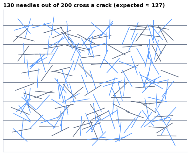
We drop a needle of length 1 on a plank floor whose cracks are 1 apart. It crosses a crack with probability (Buffon, 1733 and 1777); Laplace (1812) suggests deducing π from it: if needles out of cross a crack.
- Simulate 3,000 needles (distance from the centre to the nearest crack uniform on , angle with the cracks uniform) and estimate π. Draw the first 200: in blue those that cross a crack.
- The trap. Drawing a uniform angle on assumes that you know π! Suggest a way of drawing a uniform direction without using π (hint: a uniform point in the quarter disc, obtained by rejection).
- Why is not unbiased, whereas is unbiased for ?
Challenges (for those who have finished)
Challenge 1 — Buffon's needle, without cheating
We drop a needle of length 1 on a plank floor whose cracks are 1 apart. It crosses a crack with probability (Buffon, 1733 and 1777); Laplace (1812) suggests deducing π from it: if needles out of cross a crack.
- Simulate 3,000 needles (distance from the centre to the nearest crack uniform on , angle with the cracks uniform) and estimate π. Draw the first 200: in blue those that cross a crack.
- The trap. Drawing a uniform angle on assumes that you know π! Suggest a way of drawing a uniform direction without using π (hint: a uniform point in the quarter disc, obtained by rejection).
- Why is not unbiased, whereas is unbiased for ?
# Challenge 1: your turnShow the solution
# Challenge 1: your turn
rng = np.random.default_rng(1777)
n_needles = 3000
centre = rng.random(n_needles) / 2                  # distance from the centre to the nearest crack
# uniform direction without π: draw uniform points in the square, keep those in the quarter disc
u = rng.random((3 * n_needles, 2))
u = u[(u**2).sum(axis=1) <= 1][:n_needles]
sin_theta = u[:, 1] / np.sqrt((u**2).sum(axis=1))  # sine of the angle with the cracks
crosses = centre <= sin_theta / 2
k = crosses.sum()
pi_buffon = 2 * n_needles / k
half_buffon = 1.96 * pi_buffon * math.sqrt((pi_buffon / 2 - 1) / n_needles)   # delta method (question 3)
print(f"{k} needles out of {n_needles} cross a crack: π ≈ 2n/k = {pi_buffon:.4f} ± {half_buffon:.4f}")

# drawing: a floor of 6 planks, 200 needles
gx = rng.random(200) * 8
gy = rng.random(200) * 6
v = rng.random((600, 2)) * 2 - 1
v = v[(v**2).sum(axis=1) <= 1][:200]
v = v / np.sqrt((v**2).sum(axis=1))[:, None] / 2
y0, y1 = gy - v[:, 1], gy + v[:, 1]
crosses_plot = np.floor(y0) != np.floor(y1)
fig, ax = plt.subplots(figsize=(8, 6))
for j in range(7):
    ax.axhline(j, color=GREY, lw=1)
for i in range(200):
    ax.plot([gx[i] - v[i, 0], gx[i] + v[i, 0]], [y0[i], y1[i]], color=BLUE if crosses_plot[i] else GREY, lw=1.5)
ax.set_aspect("equal")
ax.set_xticks([])
ax.set_yticks([])
ax.grid(False)
ax.set_title(f"{crosses_plot.sum()} needles out of 200 cross a crack (expected ≈ {200 * 2 / math.pi:.0f})")
plt.show()
1872 needles out of 3000 cross a crack: π ≈ 2n/k = 3.2051 ± 0.0890
# Challenge 1: your turn
rng = np.random.default_rng(1777)
n_needles = 3000
centre = rng.random(n_needles) / 2                  # distance from the centre to the nearest crack
# uniform direction without π: draw uniform points in the square, keep those in the quarter disc
u = rng.random((3 * n_needles, 2))
u = u[(u**2).sum(axis=1) <= 1][:n_needles]
sin_theta = u[:, 1] / np.sqrt((u**2).sum(axis=1))  # sine of the angle with the cracks
crosses = centre <= sin_theta / 2
k = crosses.sum()
pi_buffon = 2 * n_needles / k
half_buffon = 1.96 * pi_buffon * math.sqrt((pi_buffon / 2 - 1) / n_needles)   # delta method (question 3)
print(f"{k} needles out of {n_needles} cross a crack: π ≈ 2n/k = {pi_buffon:.4f} ± {half_buffon:.4f}")

# drawing: a floor of 6 planks, 200 needles
gx = rng.random(200) * 8
gy = rng.random(200) * 6
v = rng.random((600, 2)) * 2 - 1
v = v[(v**2).sum(axis=1) <= 1][:200]
v = v / np.sqrt((v**2).sum(axis=1))[:, None] / 2
y0, y1 = gy - v[:, 1], gy + v[:, 1]
crosses_plot = np.floor(y0) != np.floor(y1)
fig, ax = plt.subplots(figsize=(8, 6))
for j in range(7):
    ax.axhline(j, color=GREY, lw=1)
for i in range(200):
    ax.plot([gx[i] - v[i, 0], gx[i] + v[i, 0]], [y0[i], y1[i]], color=BLUE if crosses_plot[i] else GREY, lw=1.5)
ax.set_aspect("equal")
ax.set_xticks([])
ax.set_yticks([])
ax.grid(False)
ax.set_title(f"{crosses_plot.sum()} needles out of 200 cross a crack (expected ≈ {200 * 2 / math.pi:.0f})")
plt.show()
1872 needles out of 3000 cross a crack: π ≈ 2n/k = 3.2051 ± 0.0890
3. is an unbiased estimator of , but is convex: by Jensen's inequality, (the bias is of order , negligible compared with the error of order ). The delta method gives the typical error: , that is about 0.043 for 3,000 needles, more than the darts for the same budget (0.030).
Challenge 2 — Is the dimension really invisible?
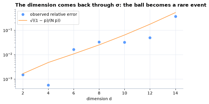
The video claims that the error “does not see the dimension”. Estimate the volume of the unit ball
of by drawing uniform points in the cube , for .
Compare with the exact volume (math.gamma) and plot the relative error
as a function of . What happens, and what becomes of the video's promise?
Challenge 2 — Is the dimension really invisible?
The video claims that the error “does not see the dimension”. Estimate the volume of the unit ball
of by drawing uniform points in the cube , for .
Compare with the exact volume (math.gamma) and plot the relative error
as a function of . What happens, and what becomes of the video's promise?
# Challenge 2: your turnShow the solution
# Challenge 2: your turn
rng = np.random.default_rng(50)
N = 100_000
dims = np.arange(2, 16, 2)
rel_err, theory_err = [], []
for d in dims:
    pts = rng.random((N, d)) * 2 - 1
    p_hat = np.mean((pts**2).sum(axis=1) <= 1)
    V = math.pi ** (d / 2) / math.gamma(d / 2 + 1)
    p = V / 2**d
    rel_err.append(abs(p_hat * 2**d - V) / V)
    theory_err.append(math.sqrt((1 - p) / (N * p)))
    print(f"d = {d:2d}: share of the cube occupied by the ball p = {p:.2e}; estimate {p_hat * 2**d:.4f}, exact {V:.4f}")
fig, ax = plt.subplots()
ax.semilogy(dims, rel_err, "o", color=BLUE, label="observed relative error")
ax.semilogy(dims, theory_err, color=ORANGE, label="√((1 − p)/(N p))")
ax.set_xlabel("dimension d")
ax.set_title("The dimension comes back through σ: the ball becomes a rare event")
ax.legend()
plt.show()
d = 2: share of the cube occupied by the ball p = 7.85e-01; estimate 3.1368, exact 3.1416 d = 4: share of the cube occupied by the ball p = 3.08e-01; estimate 4.9376, exact 4.9348 d = 6: share of the cube occupied by the ball p = 8.07e-02; estimate 5.2518, exact 5.1677 d = 8: share of the cube occupied by the ball p = 1.59e-02; estimate 3.9245, exact 4.0587 d = 10: share of the cube occupied by the ball p = 2.49e-03; estimate 2.4678, exact 2.5502 d = 12: share of the cube occupied by the ball p = 3.26e-04; estimate 1.2698, exact 1.3353 d = 14: share of the cube occupied by the ball p = 3.66e-05; estimate 0.8192, exact 0.5993
# Challenge 2: your turn
rng = np.random.default_rng(50)
N = 100_000
dims = np.arange(2, 16, 2)
rel_err, theory_err = [], []
for d in dims:
    pts = rng.random((N, d)) * 2 - 1
    p_hat = np.mean((pts**2).sum(axis=1) <= 1)
    V = math.pi ** (d / 2) / math.gamma(d / 2 + 1)
    p = V / 2**d
    rel_err.append(abs(p_hat * 2**d - V) / V)
    theory_err.append(math.sqrt((1 - p) / (N * p)))
    print(f"d = {d:2d}: share of the cube occupied by the ball p = {p:.2e}; estimate {p_hat * 2**d:.4f}, exact {V:.4f}")
fig, ax = plt.subplots()
ax.semilogy(dims, rel_err, "o", color=BLUE, label="observed relative error")
ax.semilogy(dims, theory_err, color=ORANGE, label="√((1 − p)/(N p))")
ax.set_xlabel("dimension d")
ax.set_title("The dimension comes back through σ: the ball becomes a rare event")
ax.legend()
plt.show()
d = 2: share of the cube occupied by the ball p = 7.85e-01; estimate 3.1368, exact 3.1416 d = 4: share of the cube occupied by the ball p = 3.08e-01; estimate 4.9376, exact 4.9348 d = 6: share of the cube occupied by the ball p = 8.07e-02; estimate 5.2518, exact 5.1677 d = 8: share of the cube occupied by the ball p = 1.59e-02; estimate 3.9245, exact 4.0587 d = 10: share of the cube occupied by the ball p = 2.49e-03; estimate 2.4678, exact 2.5502 d = 12: share of the cube occupied by the ball p = 3.26e-04; estimate 1.2698, exact 1.3353 d = 14: share of the cube occupied by the ball p = 3.66e-05; estimate 0.8192, exact 0.5993
The rate does not depend on , but the constant does: the relative error is , where is the share of the cube occupied by the ball, which collapses with the dimension ( for ). The ball becomes a rare event. The video's promise remains true (a grid would do much worse: points for 10 per axis), but it is about the exponent, not about . This is the Achilles' heel announced at the end of the video, and the subject of Session 3.
Challenge 3 — When the interval lies
A ruin that happens once in two hundred (). For , and simulations, measure over 2,000 repetitions the coverage rate of the interval “estimate ± 1.96 ”. What happens for ? What is the interval when no ruin is observed?
Challenge 3 — When the interval lies
A ruin that happens once in two hundred (). For , and simulations, measure over 2,000 repetitions the coverage rate of the interval “estimate ± 1.96 ”. What happens for ? What is the interval when no ruin is observed?
# Challenge 3: your turnShow the solution
# Challenge 3: your turn
rng = np.random.default_rng(200)
p = 0.005
for N in (100, 1_000, 10_000):
    k = rng.binomial(N, p, size=2000)
    ph = k / N
    h = 1.96 * np.sqrt(ph * (1 - ph) / N)
    cover = np.mean(np.abs(ph - p) <= h)
    print(f"N = {N:>6}: coverage {cover:.1%}; share of repetitions with no ruin at all: {np.mean(k == 0):.1%}")
N = 100: coverage 39.1%; share of repetitions with no ruin at all: 61.0% N = 1000: coverage 86.2%; share of repetitions with no ruin at all: 0.6% N = 10000: coverage 94.8%; share of repetitions with no ruin at all: 0.0%
# Challenge 3: your turn
rng = np.random.default_rng(200)
p = 0.005
for N in (100, 1_000, 10_000):
    k = rng.binomial(N, p, size=2000)
    ph = k / N
    h = 1.96 * np.sqrt(ph * (1 - ph) / N)
    cover = np.mean(np.abs(ph - p) <= h)
    print(f"N = {N:>6}: coverage {cover:.1%}; share of repetitions with no ruin at all: {np.mean(k == 0):.1%}")
N = 100: coverage 39.1%; share of repetitions with no ruin at all: 61.0% N = 1000: coverage 86.2%; share of repetitions with no ruin at all: 0.6% N = 10000: coverage 94.8%; share of repetitions with no ruin at all: 0.0%
For , no ruin is observed in about 60% of the repetitions (): the interval is then and does not contain . The coverage collapses, far below 95%. The central limit theorem is asymptotic: must be large (in practice, a few dozen observed events). For rare events, we will have to aim where it counts (Session 3).